Note
Click here to download the full example code
Benchmarking with MOABB showing the CO2 footprint#
This example shows how to use MOABB to track the CO2 footprint using CodeCarbon library. For this example, we will use only one dataset to keep the computation time low, but this benchmark is designed to easily scale to many datasets. Due to limitation of online documentation generation, the results is computed on a local cluster but could be easily replicated on your infrastructure.
# Authors: Igor Carrara <igor.carrara@inria.fr>
#          Bruno Aristimunha <b.aristimunha@gmail.com>
#
# License: BSD (3-clause)
from moabb import benchmark, set_log_level
from moabb.analysis.plotting import codecarbon_plot
from moabb.datasets import BNCI2014_001, Zhou2016
from moabb.paradigms import LeftRightImagery


set_log_level("info")
Loading the pipelines#
To run this example we use several pipelines, ML and DL (Keras) and also
pipelines that need an optimization of the hyperparameter.
All this different pipelines are stored in pipelines_codecarbon
Selecting the datasets (optional)#
If you want to limit your benchmark on a subset of datasets, you can use the
include_datasets and exclude_datasets arguments. You will need either
to provide the dataset’s object, or a dataset’s code. To get the list of
available dataset’s code for a given paradigm, you can use the following
command:
paradigm = LeftRightImagery()
for d in paradigm.datasets:
    print(d.code)
In this example, we will use only the last dataset, ‘Zhou 2016’, considering only the first subject.
Running the benchmark#
The benchmark is run using the benchmark function. You need to specify the
folder containing the pipelines to use, the kind of evaluation and the paradigm
to use. By default, the benchmark will use all available datasets for all
paradigms listed in the pipelines. You could restrict to specific evaluation
and paradigm using the evaluations and paradigms arguments.
To save computation time, the results are cached. If you want to re-run the
benchmark, you can set the overwrite argument to True.
It is possible to indicate the folder to cache the results and the one to
save the analysis & figures. By default, the results are saved in the
results folder, and the analysis & figures are saved in the benchmark
folder.
dataset = Zhou2016()
dataset2 = BNCI2014_001()
dataset.subject_list = dataset.subject_list[:1]
dataset2.subject_list = dataset2.subject_list[:1]
datasets = [dataset, dataset2]

results = benchmark(
    pipelines="./pipelines_codecarbon/",
    evaluations=["WithinSession"],
    paradigms=["LeftRightImagery"],
    include_datasets=datasets,
    results="./results/",
    overwrite=False,
    plot=False,
    output="./benchmark/",
)
Benchmark prints a summary of the results. Detailed results are saved in a
pandas dataframe, and can be used to generate figures. The analysis & figures
are saved in the benchmark folder.
results.head()

order_list = [
    "CSP + SVM",
    "Tangent Space LR",
    "EN Grid",
    "CSP + LDA Grid",
    "Keras_EEGNet_8_2",
]
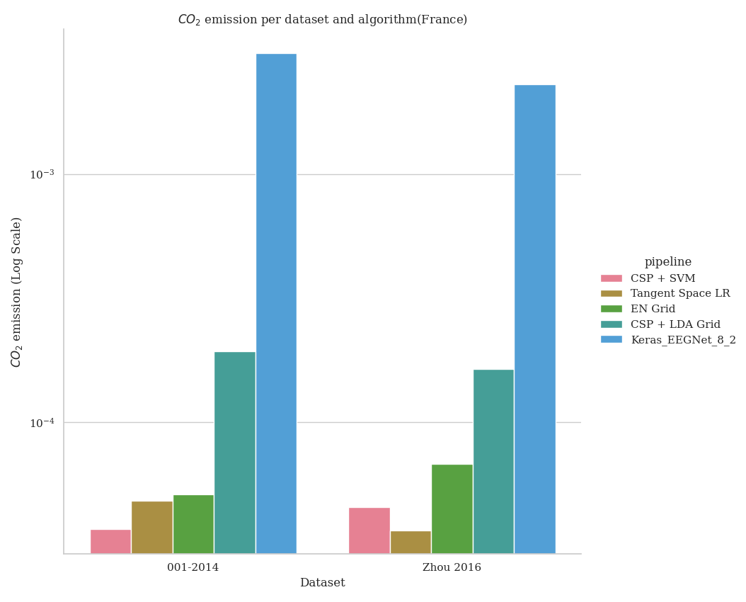
Plotting the results#
We can plot the results using the codecarbon_plot function, generated
below. This function takes the dataframe returned by the benchmark
function as input, and returns a pyplot figure.
The order_list argument is used to specify the order of the pipelines in
the plot.
codecarbon_plot(results, order_list, country="(France)")
- The result expected will be the following image, but varying depending on the
machine and the country used to run the example.
Total running time of the script: ( 0 minutes 0.000 seconds)
Estimated memory usage: 0 MB