

Note
Go to the end to download the full example code.
Trialwise cross-subject subject-prototype classification#
Minimum Distance to Mean (MDM) [1] represents each class by one Riemannian mean covariance matrix. In a cross-subject setting, pooling every source subject into one mean can hide useful subject structure.
This tutorial builds a subject-prototype MDM (SP-MDM) classifier. It learns one class prototype per source subject, routes subject identifiers to the classifier during fitting, and predicts a held-out target trial from its mean distance to those prototypes.
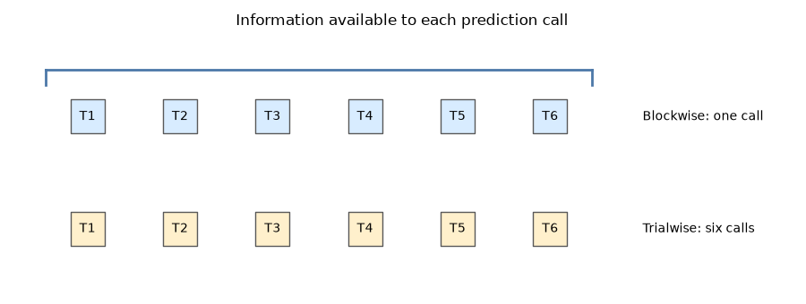
We also use MOABB’s strict TRAIN_TRIALWISE protocol. The fitted model sees
one target trial per prediction call, so it cannot estimate a normalization,
alignment, or other statistic from the complete target test block.
# Authors: Anton Andonov <toncho11@gmail.com>
#          Bruno Aristimunha <b.aristimunha@gmail.com>
#
# License: BSD (3-clause)

import matplotlib.pyplot as plt
import numpy as np
from pyriemann.classification import MDM
from pyriemann.estimation import Covariances
from pyriemann.geometry.distance import distance_riemann
from pyriemann.geometry.mean import mean_riemann
from sklearn import config_context
from sklearn.base import BaseEstimator, ClassifierMixin
from sklearn.pipeline import make_pipeline

from moabb.datasets.fake import FakeDataset
from moabb.evaluations import CrossSubjectEvaluation
from moabb.evaluations.protocols import CrossSubjectMode
from moabb.paradigms import LeftRightImagery
From one class mean to subject prototypes#
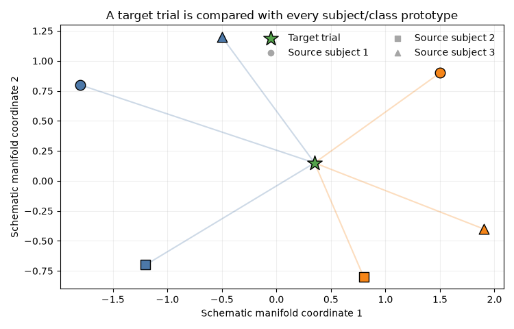
Standard MDM estimates one prototype \(G_k\) for every class \(k\) after pooling all training trials. SP-MDM instead estimates \(G_{s,k}\) for every source subject \(s\) and class \(k\).
For a new covariance matrix \(C\), its distance to class \(k\) is
where \(d_R\) is the affine-invariant Riemannian distance and \(S_k\) contains the source subjects for which class \(k\) is available. The predicted class minimizes \(D_k(C)\).
The sketch below shows why subject IDs matter. Blue and orange denote the two classes; marker shapes denote source subjects. Pooling would replace each colored set with one mean, whereas SP-MDM retains all six reference points.
prototype_xy = np.array(
    [[-1.8, 0.8], [-1.2, -0.7], [-0.5, 1.2], [1.5, 0.9], [0.8, -0.8], [1.9, -0.4]]
)
target_xy = np.array([0.35, 0.15])
prototype_class = np.array([0, 0, 0, 1, 1, 1])
markers = ["o", "s", "^"]
colors = ["#4C78A8", "#F58518"]

fig, ax = plt.subplots(figsize=(7.5, 4.8))
for index, point in enumerate(prototype_xy):
    klass = prototype_class[index]
    subject = index % 3
    ax.scatter(
        *point,
        s=110,
        marker=markers[subject],
        color=colors[klass],
        edgecolor="black",
        zorder=3,
    )
    ax.plot(
        [target_xy[0], point[0]],
        [target_xy[1], point[1]],
        color=colors[klass],
        alpha=0.28,
        linewidth=1.5,
    )

ax.scatter(
    *target_xy,
    marker="*",
    s=260,
    color="#54A24B",
    edgecolor="black",
    label="Target trial",
    zorder=4,
)
for subject, marker in enumerate(markers, start=1):
    ax.scatter([], [], marker=marker, color="0.65", label=f"Source subject {subject}")
ax.set(
    xlabel="Schematic manifold coordinate 1",
    ylabel="Schematic manifold coordinate 2",
    title="A target trial is compared with every subject/class prototype",
)
ax.legend(ncols=2, frameon=False)
ax.grid(alpha=0.2)
fig.tight_layout()
plt.show()
Implement SP-MDM as a small scikit-learn classifier#
The covariance matrices and task labels are ordinary X and y.
subjects is metadata: it identifies the domain of each training row but
is not a prediction feature. The estimator therefore exposes it only as an
optional keyword in fit and later requests it through scikit-learn’s
metadata-routing API.
decision_function returns a signed score for binary ROC AUC. A positive
value means that the covariance is closer to the second class than to the
first.
class SubjectPrototypeMDM(ClassifierMixin, BaseEstimator):
    """MDM using one class prototype per source subject."""

    def fit(self, X, y, *, subjects=None):
        if subjects is None:
            raise ValueError("SubjectPrototypeMDM needs `subjects` metadata.")

        X = np.asarray(X)
        y = np.asarray(y)
        subjects = np.asarray(subjects)
        self.classes_ = np.unique(y)
        self.prototypes_ = {
            klass: [
                mean_riemann(X[(subjects == subject) & (y == klass)])
                for subject in np.unique(subjects)
                if np.any((subjects == subject) & (y == klass))
            ]
            for klass in self.classes_
        }
        return self

    def _distances(self, X):
        return np.asarray(
            [
                [
                    np.mean([distance_riemann(cov, ref) for ref in self.prototypes_[k]])
                    for k in self.classes_
                ]
                for cov in X
            ]
        )

    def predict(self, X):
        return self.classes_[np.argmin(self._distances(X), axis=1)]

    def decision_function(self, X):
        distances = self._distances(X)
        if len(self.classes_) == 2:
            return distances[:, 0] - distances[:, 1]
        return -distances
Build a subject-aware pipeline#
Only SubjectPrototypeMDM requests subjects. Covariances remains a
standard pyRiemann transformer, and a baseline MDM pipeline requests no
metadata at all.
with config_context(enable_metadata_routing=True):
    sp_mdm = SubjectPrototypeMDM().set_fit_request(subjects=True)

pipelines = {
    "Pooled MDM": make_pipeline(Covariances("oas"), MDM(metric="riemann")),
    "Subject-prototype MDM": make_pipeline(Covariances("oas"), sp_mdm),
}
What does trialwise scoring guarantee?#
TRAIN and TRAIN_TRIALWISE expose exactly the same source information
during fitting: neither provides target calibration trials. Their difference
is the batch presented during scoring.
MOABB implements the strict mode with scikit-learn’s
FrozenEstimator,
cross_val_predict(), and
LeaveOneOut. FrozenEstimator makes every
target-side fit a no-op, while LeaveOneOut makes every prediction fold
contain one trial. The individual responses are collected before the
session-level ROC AUC is computed.
This restriction matters for a method that might otherwise compute target
batch statistics inside predict. It is redundant for a strictly inductive
estimator such as the SP-MDM implementation above, but it makes the benchmark
contract explicit and enforceable.
fig, ax = plt.subplots(figsize=(9, 3.4))
trial_x = np.arange(6)
for row, (label, color) in enumerate(
    [("Blockwise: one call", "#D8ECFF"), ("Trialwise: six calls", "#FFF0CC")]
):
    ax.scatter(
        trial_x, np.full(6, 1 - row), marker="s", s=720, color=color, edgecolor="0.35"
    )
    for trial in trial_x:
        ax.text(trial, 1 - row, f"T{trial + 1}", ha="center", va="center")
    ax.text(6.0, 1 - row, label, va="center", fontsize=10)

ax.plot([-0.45, 5.45], [1.42, 1.42], color="#4C78A8", linewidth=2)
ax.plot([-0.45, -0.45], [1.28, 1.42], color="#4C78A8", linewidth=2)
ax.plot([5.45, 5.45], [1.28, 1.42], color="#4C78A8", linewidth=2)
ax.set(xlim=(-0.8, 7.6), ylim=(-0.55, 1.75), yticks=[], xticks=[])
ax.set_title("Information available to each prediction call")
for spine in ax.spines.values():
    spine.set_visible(False)
fig.tight_layout()
plt.show()
Run a fair trialwise comparison#
Both pipelines are evaluated under the same TRAIN_TRIALWISE protocol, so
any difference comes from the classifier rather than a different target-data
budget. The deterministic fake dataset keeps the example fast and
download-free; its labels contain no meaningful physiological effect.
dataset = FakeDataset(["left_hand", "right_hand"], n_subjects=4, n_sessions=2, seed=42)
paradigm = LeftRightImagery()
evaluation = CrossSubjectEvaluation(
    paradigm=paradigm,
    datasets=[dataset],
    cs_mode=CrossSubjectMode.TRAIN_TRIALWISE,
    overwrite=True,
    suffix="subject_prototype_mdm",
)
results = evaluation.process(pipelines)

print(
    results.groupby("pipeline")["score"]
    .agg(["mean", "std", "count"])
    .sort_values("mean", ascending=False)
    .round(3)
)
                        mean    std  count
pipeline
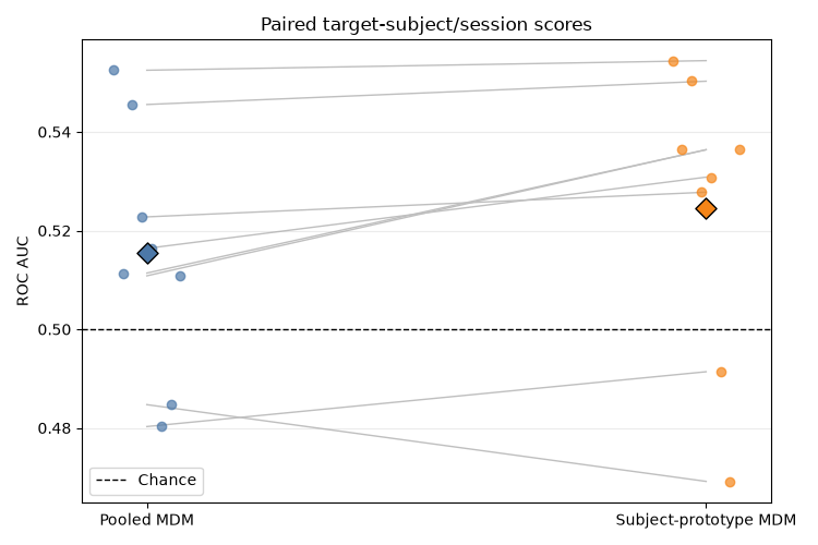
Subject-prototype MDM  0.525  0.029      8
Pooled MDM             0.516  0.026      8
Inspect paired held-out subjects#
Every gray line connects the two classifiers on the same target subject and session. Diamonds show means. Because this is fake data, both methods should fluctuate around chance and the ranking must not be interpreted as evidence.
On real datasets, use the same paired structure across many subjects and datasets, then apply MOABB’s statistical-analysis utilities. Trialwise prediction is intentionally more expensive than blockwise prediction because the frozen estimator is invoked separately for every target trial.
paired = results.pivot(index=["subject", "session"], columns="pipeline", values="score")
order = ["Pooled MDM", "Subject-prototype MDM"]
colors = ["#4C78A8", "#F58518"]

fig, ax = plt.subplots(figsize=(7.5, 5))
for row in paired[order].dropna().to_numpy():
    ax.plot([0, 1], row, color="0.75", linewidth=1, zorder=1)

for position, (pipeline, color) in enumerate(zip(order, colors, strict=True)):
    values = paired[pipeline].dropna().to_numpy()
    offsets = np.linspace(-0.06, 0.06, len(values))
    ax.scatter(position + offsets, values, color=color, alpha=0.7, zorder=2)
    ax.scatter(
        position,
        values.mean(),
        marker="D",
        s=95,
        color=color,
        edgecolor="black",
        zorder=3,
    )

ax.axhline(0.5, color="black", linestyle="--", linewidth=1, label="Chance")
ax.set(
    xticks=[0, 1],
    xticklabels=order,
    ylabel="ROC AUC",
    title="Paired target-subject/session scores",
)
ax.grid(axis="y", alpha=0.25)
ax.legend()
fig.tight_layout()
plt.show()
References#
Total running time of the script: (0 minutes 10.001 seconds)
Estimated memory usage: 487 MB
Run this example
