

Note
Go to the end to download the full example code.
Time-Resolved Decoding with SlidingEstimator#
This example shows how to perform time-resolved decoding of EEG signals using
mne.decoding.SlidingEstimator. Instead of reducing the entire trial to
a single score, a SlidingEstimator fits an independent classifier at each time
point, revealing when during a trial the neural signal carries information
about the mental state.
This approach is a natural alternative to pseudo-online evaluation (using overlapping windows): rather than simulating an online scenario by slicing the raw signal with a sliding window, we directly assess decoding accuracy at each sample of the already-epoched trial.
We use the BNCI2014-001 motor-imagery dataset (left- vs right-hand) and apply
a logistic-regression classifier wrapped in a SlidingEstimator. For each
subject the score is evaluated via stratified 5-fold cross-validation using
mne.decoding.cross_val_multiscore(), and the results are averaged across
subjects and visualised as a time course.
# Authors: MOABB contributors
#
# License: BSD (3-clause)
# sphinx_gallery_thumbnail_number = 2

import warnings

import matplotlib.pyplot as plt
import numpy as np
from mne.decoding import SlidingEstimator, cross_val_multiscore
from scipy.stats import ttest_1samp
from sklearn.linear_model import LogisticRegression
from sklearn.pipeline import make_pipeline
from sklearn.preprocessing import StandardScaler

import moabb
from moabb.datasets import BNCI2014_001
from moabb.paradigms import LeftRightImagery


moabb.set_log_level("info")
warnings.filterwarnings("ignore")
Loading the Dataset#
We instantiate the BNCI2014-001 dataset and use all 9 subjects.
dataset = BNCI2014_001()
Choosing a Paradigm#
The LeftRightImagery paradigm extracts
left-hand and right-hand motor-imagery epochs, applies a band-pass filter
(8–32 Hz by default), and returns the data as a 3-D NumPy array of shape
(n_trials, n_channels, n_times).
Building a Time-Resolved Pipeline#
A SlidingEstimator wraps any scikit-learn compatible
estimator and fits/scores it independently at every time point.
Here we use a simple logistic-regression classifier with Z-score
normalisation. The scoring='roc_auc' argument tells the estimator to
use AUC as the evaluation metric.
clf = make_pipeline(StandardScaler(), LogisticRegression(max_iter=1000))
sliding = SlidingEstimator(clf, scoring="roc_auc", n_jobs=1)
Evaluating Each Subject#
For each subject we:
Retrieve the preprocessed epochs via the paradigm using
return_epochs=Trueso we can extract the correct time vector and sampling frequency from themne.Epochsmetadata.Run stratified 5-fold cross-validation with
cross_val_multiscore(), which returns an array of shape(n_folds, n_times).Average over folds to obtain a single time course per subject.
All per-subject time courses are collected for later aggregation.
all_scores = []

for subject in dataset.subject_list:
    epochs, y, meta = paradigm.get_data(
        dataset=dataset, subjects=[subject], return_epochs=True
    )
    X = epochs.get_data()

    # cross_val_multiscore returns (n_folds, n_times)
    scores = cross_val_multiscore(sliding, X, y, cv=5, n_jobs=1)
    all_scores.append(scores.mean(axis=0))  # average over folds

# Stack into (n_subjects, n_times)
all_scores = np.array(all_scores)
This is nemar-py 0.3.3.
Preparing to download nm000139 from https://data.nemar.org/
Retrieving 6 of 769 manifest files (16 concurrent downloads).

S3:   0%|          | 0.00/85.4M [00:00<?, ?B/s]
S3:   1%|          | 1.00M/85.4M [00:00<00:35, 2.52MB/s]
S3:   7%|▋         | 6.00M/85.4M [00:00<00:05, 15.1MB/s]
S3:  27%|██▋       | 23.0M/85.4M [00:00<00:01, 56.8MB/s]
S3:  62%|██████▏   | 53.0M/85.4M [00:00<00:00, 123MB/s]
S3:  90%|████████▉ | 76.7M/85.4M [00:00<00:00, 146MB/s]
S3: 100%|██████████| 85.4M/85.4M [00:00<00:00, 97.1MB/s]
Finished downloading nm000139 v1.0.3.
Extracting the Time Vector#
Because we used return_epochs=True, we can read the time axis and
sampling frequency directly from the last Epochs object rather than
hard-coding dataset-specific values.
times = epochs.times
sfreq = epochs.info["sfreq"]
print(f"Sampling frequency: {sfreq} Hz, {len(times)} time points")
Sampling frequency: 250.0 Hz, 1001 time points
Statistical Significance#
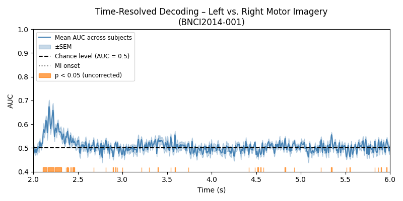
We run a one-sample t-test against chance level (AUC = 0.5) at each time point. Time points with p < 0.05 (uncorrected) are flagged as significant.
_, p_values = ttest_1samp(all_scores, 0.5, axis=0)
sig_mask = p_values < 0.05
Plot 1 – Mean AUC Time Course with Significance#
We plot the group-average AUC score together with the standard error of the mean (SEM) across subjects. A horizontal dashed line at 0.5 indicates chance level. Time points that are significantly above chance are highlighted with an orange bar along the x-axis.
mean_scores = all_scores.mean(axis=0)
sem_scores = all_scores.std(axis=0) / np.sqrt(len(dataset.subject_list))

fig, ax = plt.subplots(figsize=(8, 4))
ax.plot(times, mean_scores, label="Mean AUC across subjects", color="steelblue")
ax.fill_between(
    times,
    mean_scores - sem_scores,
    mean_scores + sem_scores,
    alpha=0.3,
    color="steelblue",
    label="\u00b1SEM",
)
ax.axhline(0.5, linestyle="--", color="k", label="Chance level (AUC = 0.5)")
ax.axvline(times[0], linestyle=":", color="gray", label="MI onset")

# Mark significant time points with a bar at the bottom of the axes
ax.fill_between(
    times,
    0.0,
    0.03,
    where=sig_mask,
    color="tab:orange",
    alpha=0.7,
    label="p < 0.05 (uncorrected)",
    transform=ax.get_xaxis_transform(),
)

ax.set_xlabel("Time (s)")
ax.set_ylabel("AUC")
ax.set_title("Time-Resolved Decoding \u2013 Left vs. Right Motor Imagery\n(BNCI2014-001)")
ax.legend(loc="upper left", fontsize="small")
ax.set_xlim(times[0], times[-1])
ax.set_ylim(0.4, 1.0)
plt.tight_layout()
plt.show()
Plot 2 – Per-Subject Heatmap#
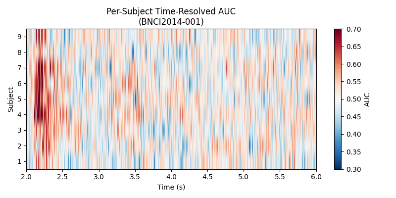
A heatmap of AUC scores (subjects x time) gives a richer picture than the mean curve alone, revealing inter-subject variability and the temporal structure of discriminability for each participant.
fig, ax = plt.subplots(figsize=(8, 4))
im = ax.imshow(
    all_scores,
    aspect="auto",
    origin="lower",
    extent=[times[0], times[-1], 0.5, len(dataset.subject_list) + 0.5],
    cmap="RdBu_r",
    vmin=0.3,
    vmax=0.7,
)
ax.set_xlabel("Time (s)")
ax.set_ylabel("Subject")
ax.set_yticks(range(1, len(dataset.subject_list) + 1))
ax.set_title("Per-Subject Time-Resolved AUC\n(BNCI2014-001)")
ax.axvline(times[0], linestyle=":", color="k", linewidth=0.8)
ax.set_xlim(times[0], times[-1])
fig.colorbar(im, ax=ax, label="AUC")
plt.tight_layout()
plt.show()
Total running time of the script: (8 minutes 38.138 seconds)
Estimated memory usage: 888 MB
Run this example
