

Note
Go to the end to download the full example code.
Tutorial 1: Simple Motor Imagery#
In this example, we will go through all the steps to make a simple BCI classification task, downloading a dataset and using a standard classifier. We choose the dataset 2a from BCI Competition IV, a motor imagery task. We will use a CSP to enhance the signal-to-noise ratio of the EEG epochs and a LDA to classify these signals.
# Authors: Pedro L. C. Rodrigues, Sylvain Chevallier
#
# https://github.com/plcrodrigues/Workshop-MOABB-BCI-Graz-2019

import warnings

import matplotlib.pyplot as plt
import pandas as pd
import seaborn as sns
from mne.decoding import CSP
from sklearn.discriminant_analysis import LinearDiscriminantAnalysis as LDA
from sklearn.pipeline import make_pipeline

import moabb
from moabb.datasets import BNCI2014_001
from moabb.evaluations import WithinSessionEvaluation
from moabb.paradigms import LeftRightImagery


moabb.set_log_level("info")
warnings.filterwarnings("ignore")
/home/runner/work/moabb/moabb/.venv/lib/python3.11/site-packages/optuna/integration/sklearn.py:14: FutureWarning: `optuna.integration.sklearn` has been deprecated in v4.9.0. This feature will be removed in v6.0.0. See https://github.com/optuna/optuna/releases/tag/v4.9.0. Use `optuna_integration.sklearn` instead.
  optuna_warn(f"{msg} Use `optuna_integration.sklearn` instead.", FutureWarning)
Instantiating Dataset#
The first thing to do is to instantiate the dataset that we want to analyze. MOABB has a list of many different datasets, each one containing all the necessary information for describing them, such as the number of subjects, size of trials, names of classes, etc.
The dataset class has methods for:
downloading its files from some online source (e.g. Zenodo)
importing the data from the files in whatever extension they might be (like .mat, .gdf, etc.) and instantiate a Raw object from the MNE package
dataset = BNCI2014_001()
dataset.subject_list = [1, 2, 3]
Accessing EEG Recording#
As an example, we may access the EEG recording from a given session and a given run as follows:
sessions = dataset.get_data(subjects=[1])
This returns a MNE Raw object that can be manipulated. This might be enough for some users, since the pre-processing and epoching steps can be easily done via MNE. However, to conduct an assessment of several classifiers on multiple subjects, MOABB ends up being a more appropriate option.
subject = 1
session_name = "0train"
run_name = "0"
raw = sessions[subject][session_name][run_name]
Choosing a Paradigm#
Once we have instantiated a dataset, we have to choose a paradigm. This object is responsible for filtering the data, epoching it, and extracting the labels for each epoch. Note that each dataset comes with the names of the paradigms to which it might be associated. It would not make sense to process a P300 dataset with a MI paradigm object.
print(dataset.paradigm)
imagery
For the example below, we will consider the paradigm associated to left-hand/right-hand motor imagery task, but there are other options in MOABB for motor imagery, P300 or SSVEP.
We may check the list of all datasets available in MOABB for using with this paradigm (note that BNCI2014_001 is in it)
print(paradigm.datasets)
[BNCI2014-001, BNCI2014-004, Beetl2021-A, Beetl2021-B, Brandl2020, Chang2025, Cho2017, Dreyer2023, Dreyer2023A, Dreyer2023B, Dreyer2023C, Forenzo2023, GrosseWentrup2009, GuttmannFlury2025-ME, GuttmannFlury2025-MI, HefmiIch2025, Kaya2018, Kumar2024, Lee2019-MI, Liu2024, PhysionetMotorImagery, Schirrmeister2017, Shin2017A, Stieger2021, Wairagkar2018, Weibo2014, Wu2020, Yang2025, Zhou2016, Zhou2020]
The data from a list of subjects could be preprocessed and return as a 3D numpy array X, follow a scikit-like format with the associated labels. The meta object contains all information regarding the subject, the session and the run associated to each trial.
Create Pipeline#
Our goal is to evaluate the performance of a given classification pipeline (or several of them) when it is applied to the epochs from the previously chosen dataset. We will consider a very simple classification pipeline in which the dimension of the epochs are reduced via a CSP step and then classified via a linear discriminant analysis.
pipeline = make_pipeline(CSP(n_components=8), LDA())
Evaluation#
To evaluate the score of this pipeline, we use the evaluation class. When instantiating it, we say which paradigm we want to consider, a list with the datasets to analyze, and whether the scores should be recalculated each time we run the evaluation or if MOABB should create a cache file.
Note that there are different ways of evaluating a classifier; in this example, we choose WithinSessionEvaluation, which consists of doing a cross-validation procedure where the training and testing partitions are from the same recording session of the dataset. We could have used CrossSessionEvaluation, which takes all but one session as training partition and the remaining one as testing partition.
evaluation = WithinSessionEvaluation(
    paradigm=paradigm, datasets=[dataset], overwrite=True, hdf5_path=None
)
We obtain the results in the form of a pandas dataframe
results = evaluation.process({"csp+lda": pipeline})
[codecarbon WARNING @ 23:35:44] Multiple instances of codecarbon are allowed to run at the same time.
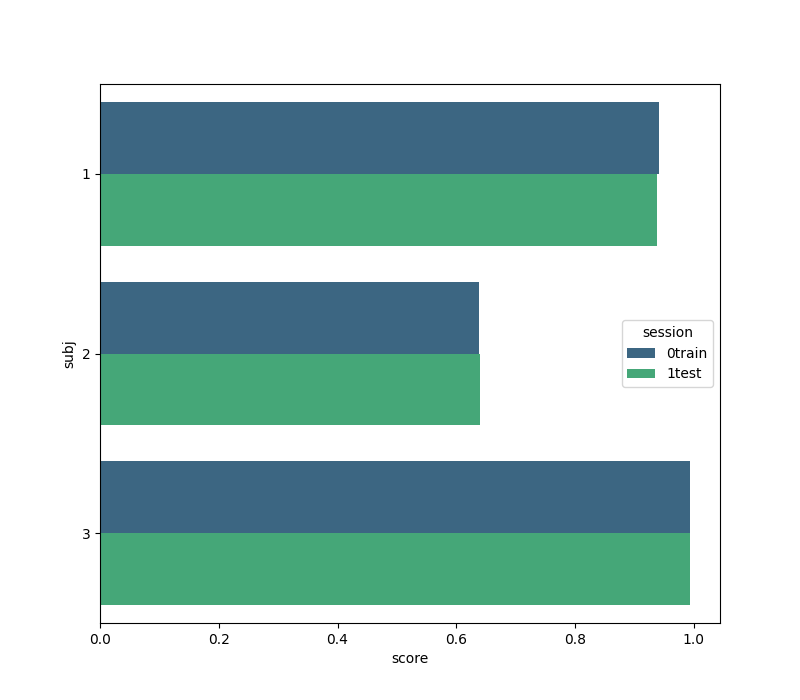
2026-07-14 23:37:21,239 INFO MainThread moabb.evaluations.base csp+lda | BNCI2014-001 | 1 | 1test: Score 0.947
2026-07-14 23:37:21,239 INFO MainThread moabb.evaluations.base csp+lda | BNCI2014-001 | 1 | 0train: Score 0.941
2026-07-14 23:37:21,239 INFO MainThread moabb.evaluations.base csp+lda | BNCI2014-001 | 2 | 1test: Score 0.673
2026-07-14 23:37:21,239 INFO MainThread moabb.evaluations.base csp+lda | BNCI2014-001 | 2 | 0train: Score 0.644
2026-07-14 23:37:21,239 INFO MainThread moabb.evaluations.base csp+lda | BNCI2014-001 | 3 | 0train: Score 0.996
2026-07-14 23:37:21,239 INFO MainThread moabb.evaluations.base csp+lda | BNCI2014-001 | 3 | 1test: Score 0.996
The results are stored in locally, to avoid recomputing the results each time. It is saved in hdf5_path if defined or in ~/mne_data/results otherwise. To export the results in CSV:
results.to_csv("./results_part2-1.csv")
To load previously obtained results saved in CSV
results = pd.read_csv("./results_part2-1.csv")
Plotting Results#
We create a figure with the seaborn package comparing the classification score for each subject on each session. Note that the ‘subject’ field from the results is given in terms of integers, but seaborn accepts only strings for its labeling. This is why we create the field ‘subj’.
2026-07-14 23:37:21,275 INFO MainThread matplotlib.category Using categorical units to plot a list of strings that are all parsable as floats or dates. If these strings should be plotted as numbers, cast to the appropriate data type before plotting.
2026-07-14 23:37:21,278 INFO MainThread matplotlib.category Using categorical units to plot a list of strings that are all parsable as floats or dates. If these strings should be plotted as numbers, cast to the appropriate data type before plotting.
Total running time of the script: (1 minutes 54.085 seconds)
Run this example