Within Session Motor Imagery with Learning Curve

This example shows how to perform a within session motor imagery analysis on the very popular dataset 2a from the BCI competition IV.

We will compare two pipelines :

• CSP + LDA

• Riemannian Geometry + Logistic Regression

We will use the LeftRightImagery paradigm. This will restrict the analysis to two classes (left- vs right-hand) and use AUC as metric.

# Original author: Alexandre Barachant <alexandre.barachant@gmail.com>
# Learning curve modification: Jan Sosulski
#
# License: BSD (3-clause)

import matplotlib.pyplot as plt
import numpy as np
import seaborn as sns
from mne.decoding import CSP
from pyriemann.estimation import Covariances
from pyriemann.tangentspace import TangentSpace
from sklearn.discriminant_analysis import LinearDiscriminantAnalysis as LDA
from sklearn.linear_model import LogisticRegression
from sklearn.pipeline import make_pipeline

import moabb
from moabb.datasets import BNCI2014_001
from moabb.evaluations import WithinSessionEvaluation
from moabb.evaluations.splitters import LearningCurveSplitter
from moabb.paradigms import LeftRightImagery


moabb.set_log_level("info")

Create Pipelines

Pipelines must be a dict of sklearn pipeline transformer.

The CSP implementation from MNE is used. We selected 8 CSP components, as usually done in the literature.

The Riemannian geometry pipeline consists in covariance estimation, tangent space mapping and finally a logistic regression for the classification.

pipelines = {}

pipelines["CSP+LDA"] = make_pipeline(
    CSP(n_components=8), LDA(solver="lsqr", shrinkage="auto")
)

pipelines["RG+LR"] = make_pipeline(
    Covariances(), TangentSpace(), LogisticRegression(solver="lbfgs")
)

Evaluation

We define the paradigm (LeftRightImagery) and the dataset (BNCI2014_001). The evaluation will return a DataFrame containing a single AUC score for each subject / session of the dataset, and for each pipeline.

Results are saved into the database, so that if you add a new pipeline, it will not run again the evaluation unless a parameter has changed. Results can be overwritten if necessary.

paradigm = LeftRightImagery()
dataset = BNCI2014_001()
dataset.subject_list = dataset.subject_list[:1]
datasets = [dataset]
overwrite = True  # set to True if we want to overwrite cached results
# Evaluate for a specific number of training samples per class
data_size = {"policy": "per_class", "value": np.array([5, 10, 30, 50])}
# When the training data is sparse, perform more permutations than when we have a lot of data
n_perms = np.floor(np.geomspace(20, 2, len(data_size["value"]))).astype(int)
evaluation = WithinSessionEvaluation(
    paradigm=paradigm,
    datasets=datasets,
    suffix="examples",
    overwrite=overwrite,
    cv_class=LearningCurveSplitter,
    cv_kwargs={"data_size": data_size, "n_perms": n_perms},
)

results = evaluation.process(pipelines)

print(results.head())

      score      time  ...  pipeline                  codecarbon_task_name
0  0.795238  0.011141  ...     RG+LR  c3f97593-4807-4033-ba82-3f8abc570c56
1  0.819048  0.016275  ...     RG+LR  7024cc1f-ff1f-4fb1-a20e-78ceadeab232
2  0.928571  0.043251  ...     RG+LR  f629d491-26d9-412f-bcc4-25f2db25b6f1
3  0.942857  0.064588  ...     RG+LR  a9dca84d-165a-4a60-9e86-914fab6a8e6e
4  0.861905  0.011062  ...     RG+LR  761d2fe2-185f-4ead-a796-df598c26eb18

[5 rows x 15 columns]

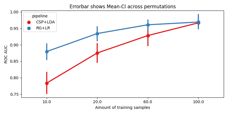
Plot Results

We plot the accuracy as a function of the number of training samples, for each pipeline

fig, ax = plt.subplots(facecolor="white", figsize=[8, 4])

n_subs = len(dataset.subject_list)

if n_subs > 1:
    r = results.groupby(["pipeline", "subject", "data_size"]).mean().reset_index()
else:
    r = results

sns.pointplot(data=r, x="data_size", y="score", hue="pipeline", ax=ax, palette="Set1")

errbar_meaning = "subjects" if n_subs > 1 else "permutations"
title_str = f"Errorbar shows Mean-CI across {errbar_meaning}"
ax.set_xlabel("Amount of training samples")
ax.set_ylabel("ROC AUC")
ax.set_title(title_str)
fig.tight_layout()
plt.show()