Within Session SSVEP

This Example shows how to perform a within-session SSVEP analysis on the MAMEM dataset 3, using a CCA pipeline.

The within-session evaluation assesses the performance of a classification pipeline using a 5-fold cross-validation. The reported metric (here, accuracy) is the average of all fold.

# Authors: Sylvain Chevallier <sylvain.chevallier@uvsq.fr>
#
# License: BSD (3-clause)

import warnings

import matplotlib.pyplot as plt
import seaborn as sns
from sklearn.pipeline import make_pipeline

import moabb
from moabb.datasets import Kalunga2016
from moabb.evaluations import WithinSessionEvaluation
from moabb.paradigms import SSVEP
from moabb.pipelines import SSVEP_CCA


warnings.simplefilter(action="ignore", category=FutureWarning)
warnings.simplefilter(action="ignore", category=RuntimeWarning)
moabb.set_log_level("info")

Loading Dataset

Load 2 subjects of Kalunga2016 dataset

subj = [1, 3]
dataset = Kalunga2016()
dataset.subject_list = subj

Choose Paradigm

We select the paradigm SSVEP, applying a bandpass filter (3-15 Hz) on the data and we keep only the first 3 classes, that is stimulation frequency of 13Hz, 17Hz and 21Hz.

paradigm = SSVEP(fmin=10, fmax=40, n_classes=3)

Create Pipelines

Use a Canonical Correlation Analysis classifier

interval = dataset.interval
freqs = paradigm.used_events(dataset)

pipeline = {}
pipeline["CCA"] = make_pipeline(SSVEP_CCA(n_harmonics=3))

Get Data (optional)

To get access to the EEG signals downloaded from the dataset, you could use dataset.get_data(subjects=[subject_id]) to obtain the EEG under MNE format, stored in a dictionary of sessions and runs. Otherwise, paradigm.get_data(dataset=dataset, subjects=[subject_id]) allows to obtain the EEG data in scikit format, the labels and the meta information. In paradigm.get_data, the EEG are preprocessed according to the paradigm requirement.

# sessions = dataset.get_data(subjects=[3])
# X, labels, meta = paradigm.get_data(dataset=dataset, subjects=[3])

Evaluation

The evaluation will return a DataFrame containing a single AUC score for each subject and pipeline.

overwrite = True  # set to True if we want to overwrite cached results

evaluation = WithinSessionEvaluation(
    paradigm=paradigm, datasets=dataset, suffix="examples", overwrite=overwrite
)
results = evaluation.process(pipeline)

print(results.head())

Kalunga2016-WithinSession:   0%|          | 0/2 [00:00<?, ?it/s]
Kalunga2016-WithinSession:  50%|█████     | 1/2 [00:06<00:06,  6.56s/it]

  0%|                                              | 0.00/2.27M [00:00<?, ?B/s]

  0%|                                     | 1.02k/2.27M [00:00<05:41, 6.66kB/s]

  2%|▋                                     | 41.0k/2.27M [00:00<00:13, 168kB/s]

  4%|█▌                                    | 95.2k/2.27M [00:00<00:07, 273kB/s]

  8%|██▉                                    | 172k/2.27M [00:00<00:05, 389kB/s]

 17%|██████▍                                | 376k/2.27M [00:00<00:02, 793kB/s]

 35%|█████████████                         | 784k/2.27M [00:00<00:00, 1.55MB/s]

 71%|██████████████████████████           | 1.60M/2.27M [00:00<00:00, 3.04MB/s]

  0%|                                              | 0.00/2.27M [00:00<?, ?B/s]
100%|█████████████████████████████████████| 2.27M/2.27M [00:00<00:00, 8.45GB/s]


  0%|                                              | 0.00/2.13M [00:00<?, ?B/s]

  1%|▏                                    | 12.3k/2.13M [00:00<00:27, 77.2kB/s]

  2%|▋                                     | 39.9k/2.13M [00:00<00:14, 146kB/s]

  4%|█▋                                    | 93.2k/2.13M [00:00<00:08, 253kB/s]

  8%|███▎                                   | 178k/2.13M [00:00<00:04, 395kB/s]

 18%|███████▏                               | 393k/2.13M [00:00<00:02, 814kB/s]

 38%|██████████████▍                       | 809k/2.13M [00:00<00:00, 1.56MB/s]

 77%|████████████████████████████▌        | 1.64M/2.13M [00:00<00:00, 3.03MB/s]

  0%|                                              | 0.00/2.13M [00:00<?, ?B/s]
100%|█████████████████████████████████████| 2.13M/2.13M [00:00<00:00, 9.00GB/s]

Kalunga2016-WithinSession: 100%|██████████| 2/2 [00:16<00:00,  8.45s/it]
Kalunga2016-WithinSession: 100%|██████████| 2/2 [00:16<00:00,  8.17s/it]
      score      time  ...  pipeline                  codecarbon_task_name
0  0.333333  0.001185  ...       CCA  1b224ea8-7736-4fe9-a3e6-2bd846fa48cc
1  0.331111  0.001121  ...       CCA  9a77c79b-fc91-41e2-9b85-df954f85d51e

[2 rows x 11 columns]

Plot Results

Here we plot the results, indicating the score for each subject

plt.figure()
sns.barplot(data=results, y="score", x="session", hue="subject", palette="viridis")

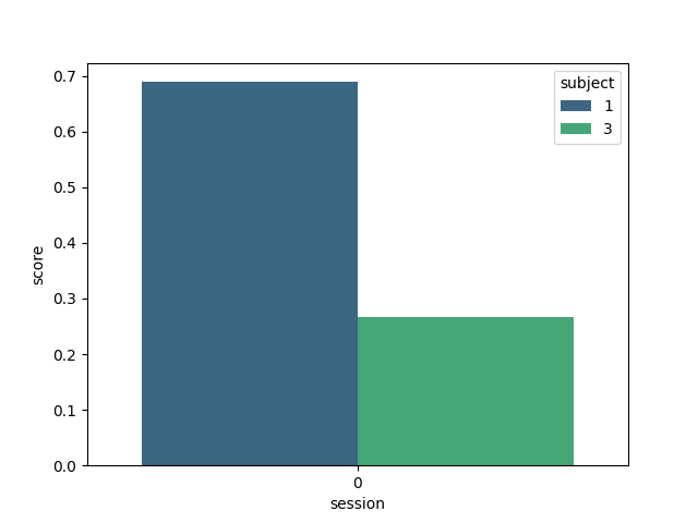
<Axes: xlabel='session', ylabel='score'>

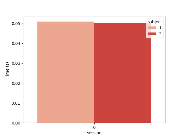
And the computation time in seconds

plt.figure()
ax = sns.barplot(data=results, y="time", x="session", hue="subject", palette="Reds")
ax.set_ylabel("Time (s)")
plt.show()

Estimated memory usage: 317 MB