Within Session P300 with Learning Curve

This example shows how to perform a within session analysis while also creating learning curves for a P300 dataset.

We will compare two pipelines :

• Riemannian geometry with Linear Discriminant Analysis

• XDAWN and Linear Discriminant Analysis

We will use the P300 paradigm, which uses the AUC as metric.

# Authors: Jan Sosulski
#
# License: BSD (3-clause)

import warnings

import matplotlib.pyplot as plt
import numpy as np
import seaborn as sns
from mne.decoding import Vectorizer
from pyriemann.estimation import XdawnCovariances
from pyriemann.spatialfilters import Xdawn
from pyriemann.tangentspace import TangentSpace
from sklearn.discriminant_analysis import LinearDiscriminantAnalysis as LDA
from sklearn.pipeline import make_pipeline

import moabb
from moabb.datasets import BNCI2014_009
from moabb.evaluations import WithinSessionEvaluation
from moabb.paradigms import P300


# getting rid of the warnings about the future (on s'en fout !)
warnings.simplefilter(action="ignore", category=FutureWarning)
warnings.simplefilter(action="ignore", category=RuntimeWarning)

moabb.set_log_level("info")

Create Pipelines

Pipelines must be a dict of sklearn pipeline transformer.

processing_sampling_rate = 128
pipelines = {}

We have to do this because the classes are called ‘Target’ and ‘NonTarget’ but the evaluation function uses a LabelEncoder, transforming them to 0 and 1

labels_dict = {"Target": 1, "NonTarget": 0}

# Riemannian geometry based classification
pipelines["RG+LDA"] = make_pipeline(
    XdawnCovariances(nfilter=5, estimator="lwf", xdawn_estimator="scm"),
    TangentSpace(),
    LDA(solver="lsqr", shrinkage="auto"),
)

pipelines["Xdw+LDA"] = make_pipeline(
    Xdawn(nfilter=2, estimator="scm"), Vectorizer(), LDA(solver="lsqr", shrinkage="auto")
)

Evaluation

We define the paradigm (P300) and use all three datasets available for it. The evaluation will return a DataFrame containing AUCs for each permutation and dataset size.

paradigm = P300(resample=processing_sampling_rate)
dataset = BNCI2014_009()
# Remove the slicing of the subject list to evaluate multiple subjects
dataset.subject_list = dataset.subject_list[1:2]
datasets = [dataset]
overwrite = True  # set to True if we want to overwrite cached results
data_size = dict(policy="ratio", value=np.geomspace(0.02, 1, 4))
# When the training data is sparse, perform more permutations than when we have a lot of data
n_perms = np.floor(np.geomspace(20, 2, len(data_size["value"]))).astype(int)
# Guarantee reproducibility
np.random.seed(7536298)
evaluation = WithinSessionEvaluation(
    paradigm=paradigm,
    datasets=datasets,
    data_size=data_size,
    n_perms=n_perms,
    suffix="examples_lr",
    overwrite=overwrite,
)

results = evaluation.process(pipelines)

BNCI2014-009-WithinSession:   0%|          | 0/1 [00:00<?, ?it/s]
BNCI2014-009-WithinSession: 100%|██████████| 1/1 [00:58<00:00, 58.34s/it]
BNCI2014-009-WithinSession: 100%|██████████| 1/1 [00:58<00:00, 58.34s/it]

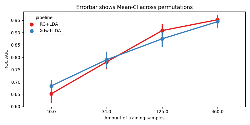
Plot Results

We plot the accuracy as a function of the number of training samples, for each pipeline

fig, ax = plt.subplots(facecolor="white", figsize=[8, 4])

n_subs = len(dataset.subject_list)

if n_subs > 1:
    r = results.groupby(["pipeline", "subject", "data_size"]).mean().reset_index()
else:
    r = results

sns.pointplot(data=r, x="data_size", y="score", hue="pipeline", ax=ax, palette="Set1")

errbar_meaning = "subjects" if n_subs > 1 else "permutations"
title_str = f"Errorbar shows Mean-CI across {errbar_meaning}"
ax.set_xlabel("Amount of training samples")
ax.set_ylabel("ROC AUC")
ax.set_title(title_str)
fig.tight_layout()
plt.show()

Estimated memory usage: 253 MB