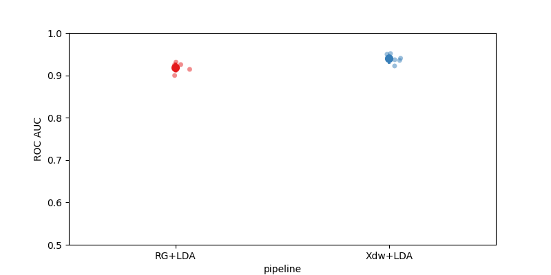
Within Session P300

This example shows how to perform a within session analysis on three different P300 datasets.

We will compare two pipelines :

• Riemannian geometry

• XDAWN with Linear Discriminant Analysis

We will use the P300 paradigm, which uses the AUC as metric.

# Authors: Pedro Rodrigues <pedro.rodrigues01@gmail.com>
#
# License: BSD (3-clause)

import warnings

import matplotlib.pyplot as plt
import seaborn as sns
from mne.decoding import Vectorizer
from pyriemann.estimation import Xdawn, XdawnCovariances
from pyriemann.tangentspace import TangentSpace
from sklearn.discriminant_analysis import LinearDiscriminantAnalysis as LDA
from sklearn.pipeline import make_pipeline

import moabb
from moabb.datasets import BNCI2014_009
from moabb.evaluations import WithinSessionEvaluation
from moabb.paradigms import P300

getting rid of the warnings about the future

warnings.simplefilter(action="ignore", category=FutureWarning)
warnings.simplefilter(action="ignore", category=RuntimeWarning)

moabb.set_log_level("info")

Create Pipelines

Pipelines must be a dict of sklearn pipeline transformer.

pipelines = {}

We have to do this because the classes are called ‘Target’ and ‘NonTarget’ but the evaluation function uses a LabelEncoder, transforming them to 0 and 1

labels_dict = {"Target": 1, "NonTarget": 0}

pipelines["RG+LDA"] = make_pipeline(
    XdawnCovariances(
        nfilter=2, classes=[labels_dict["Target"]], estimator="lwf", xdawn_estimator="scm"
    ),
    TangentSpace(),
    LDA(solver="lsqr", shrinkage="auto"),
)

pipelines["Xdw+LDA"] = make_pipeline(
    Xdawn(nfilter=2, estimator="scm"), Vectorizer(), LDA(solver="lsqr", shrinkage="auto")
)

Evaluation

We define the paradigm (P300) and use all three datasets available for it. The evaluation will return a DataFrame containing a single AUC score for each subject / session of the dataset, and for each pipeline.

Results are saved into the database, so that if you add a new pipeline, it will not run again the evaluation unless a parameter has changed. Results can be overwritten if necessary.

paradigm = P300(resample=128)
dataset = BNCI2014_009()
dataset.subject_list = dataset.subject_list[:2]
datasets = [dataset]
overwrite = True  # set to True if we want to overwrite cached results
evaluation = WithinSessionEvaluation(
    paradigm=paradigm, datasets=datasets, suffix="examples", overwrite=overwrite
)
results = evaluation.process(pipelines)

BNCI2014-009-WithinSession:   0%|          | 0/2 [00:00<?, ?it/s]

  0%|                                              | 0.00/18.5M [00:00<?, ?B/s]

  0%|                                     | 8.19k/18.5M [00:00<03:48, 81.1kB/s]

  0%|                                      | 56.3k/18.5M [00:00<00:59, 311kB/s]

  1%|▎                                      | 144k/18.5M [00:00<00:32, 562kB/s]

  2%|▋                                     | 329k/18.5M [00:00<00:17, 1.05MB/s]

  4%|█▍                                    | 696k/18.5M [00:00<00:09, 1.97MB/s]

  8%|██▊                                  | 1.42M/18.5M [00:00<00:04, 3.71MB/s]

 16%|█████▊                               | 2.88M/18.5M [00:00<00:02, 7.14MB/s]

 26%|█████████▊                           | 4.90M/18.5M [00:00<00:01, 11.2MB/s]

 38%|██████████████                       | 7.02M/18.5M [00:00<00:00, 14.1MB/s]

 50%|██████████████████▍                  | 9.26M/18.5M [00:01<00:00, 16.5MB/s]

 63%|███████████████████████▏             | 11.6M/18.5M [00:01<00:00, 18.4MB/s]

 76%|████████████████████████████         | 14.1M/18.5M [00:01<00:00, 20.1MB/s]

 90%|█████████████████████████████████▏   | 16.6M/18.5M [00:01<00:00, 21.7MB/s]

  0%|                                              | 0.00/18.5M [00:00<?, ?B/s]
100%|█████████████████████████████████████| 18.5M/18.5M [00:00<00:00, 65.9GB/s]

BNCI2014-009-WithinSession:  50%|█████     | 1/2 [00:10<00:10, 10.04s/it]

  0%|                                              | 0.00/18.5M [00:00<?, ?B/s]

  0%|                                     | 8.19k/18.5M [00:00<03:47, 81.3kB/s]

  0%|                                      | 56.3k/18.5M [00:00<00:59, 311kB/s]

  1%|▎                                      | 153k/18.5M [00:00<00:30, 599kB/s]

  2%|▋                                     | 344k/18.5M [00:00<00:16, 1.10MB/s]

  4%|█▌                                    | 736k/18.5M [00:00<00:08, 2.08MB/s]

  8%|███                                  | 1.50M/18.5M [00:00<00:04, 3.92MB/s]

 16%|██████                               | 3.06M/18.5M [00:00<00:02, 7.58MB/s]

 27%|██████████▏                          | 5.09M/18.5M [00:00<00:01, 11.5MB/s]

 38%|██████████████                       | 7.02M/18.5M [00:00<00:00, 13.8MB/s]

 49%|██████████████████▏                  | 9.08M/18.5M [00:01<00:00, 15.7MB/s]

 60%|██████████████████████               | 11.0M/18.5M [00:01<00:00, 16.8MB/s]

 71%|██████████████████████████▏          | 13.1M/18.5M [00:01<00:00, 17.8MB/s]

 82%|██████████████████████████████▎      | 15.2M/18.5M [00:01<00:00, 18.5MB/s]

 93%|██████████████████████████████████▎  | 17.2M/18.5M [00:01<00:00, 18.9MB/s]

  0%|                                              | 0.00/18.5M [00:00<?, ?B/s]
100%|█████████████████████████████████████| 18.5M/18.5M [00:00<00:00, 68.5GB/s]

BNCI2014-009-WithinSession: 100%|██████████| 2/2 [00:20<00:00, 10.19s/it]
BNCI2014-009-WithinSession: 100%|██████████| 2/2 [00:20<00:00, 10.17s/it]

Plot Results

Here we plot the results to compare the two pipelines

fig, ax = plt.subplots(facecolor="white", figsize=[8, 4])

sns.stripplot(
    data=results,
    y="score",
    x="pipeline",
    ax=ax,
    jitter=True,
    alpha=0.5,
    zorder=1,
    palette="Set1",
)
sns.pointplot(data=results, y="score", x="pipeline", ax=ax, palette="Set1")

ax.set_ylabel("ROC AUC")
ax.set_ylim(0.5, 1)

plt.show()

Estimated memory usage: 313 MB