Pipelines using the mne-features library

This example shows how to evaluate a pipeline constructed using the mne-features library [1]. This library provides sklearn compatible feature extractors for M/EEG data. These features can be used directly in your pipelines.

A list of available features can be found in the docs.

Be sure to install mne-features by running pip install mne-features.

# Authors: Alexander de Ranitz <alexanderderanitz@gmail.com>
#          Luuk Neervens <luuk.neervens@ru.nl>
#          Charlynn van Osch <charlynn.vanosch@ru.nl>
#
# License: BSD (3-clause)

import warnings

import matplotlib.pyplot as plt
import mne
import seaborn as sns
from mne_features.feature_extraction import FeatureExtractor
from sklearn.discriminant_analysis import LinearDiscriminantAnalysis as LDA
from sklearn.pipeline import make_pipeline

import moabb
from moabb.datasets import BNCI2014_001
from moabb.evaluations import WithinSessionEvaluation
from moabb.paradigms import LeftRightImagery


mne.set_log_level("CRITICAL")
moabb.set_log_level("info")
warnings.filterwarnings("ignore")

Creating Pipelines using mne-features

Here, we closely follow Tutorial 3, but we create pipelines using features extracted using the mne-features library [1]. We instantiate the three different classiciation pipelines to be considered in the analysis. See the mne-features docs to learn more about the available features: https://mne.tools/mne-features/api.html#api-documentation

Feature Details

We will use the FeatureExtractor to compute features. Here, we select two simple features: variance and ptp_amp (peak-to-peak amplitude).

Variance: Computed per channel (c). It measures the spread of the signal values (samples in vector x) around their average value (mean(x)). It involves summing the squared differences between each sample and the mean, then normalizing, at mne-features, it is the number of samples minus 1.

Peak-to-Peak Amplitude (ptp_amp): Computed per channel (c). This is simply the difference between the maximum and minimum signal values found within that channel’s data vector x. Formula: ptp_amp(c) = max(x) - min(x)

sfreq = 250.0  # sampling frequency used in the datasets below

variance = FeatureExtractor(sfreq, ["variance"])
ptp_amp = FeatureExtractor(sfreq, ["ptp_amp"])

# We can also extract several features by passing more than one feature.
both = FeatureExtractor(sfreq, ["ptp_amp", "variance"])

Pipelines with FeatureExtractor

The FeatureExtractor from mne-features is scikit-learn compatible and can therefore be used directly in our pipelines. Here, these transformer steps perform feature extraction, reducing the dimensionality of the data. We train an LDA classifier to classify our data as left- or right hand based on the extracted signal.

pipelines = {}
pipelines["var+LDA"] = make_pipeline(variance, LDA())
pipelines["ptp_amp+LDA"] = make_pipeline(ptp_amp, LDA())
pipelines["var+ptp_amp+LDA"] = make_pipeline(both, LDA())

The rest is the same as in previous tutorials!

datasets = [BNCI2014_001()]
subj = [1, 2, 3]
for d in datasets:
    d.subject_list = subj
paradigm = LeftRightImagery()
evaluation = WithinSessionEvaluation(
    paradigm=paradigm, datasets=datasets, overwrite=False
)
results = evaluation.process(pipelines)

BNCI2014-001-WithinSession:   0%|          | 0/3 [00:00<?, ?it/s]No hdf5_path provided, models will not be saved.
No hdf5_path provided, models will not be saved.
No hdf5_path provided, models will not be saved.
No hdf5_path provided, models will not be saved.
No hdf5_path provided, models will not be saved.
No hdf5_path provided, models will not be saved.

BNCI2014-001-WithinSession:  33%|███▎      | 1/3 [00:07<00:14,  7.47s/it]No hdf5_path provided, models will not be saved.
No hdf5_path provided, models will not be saved.
No hdf5_path provided, models will not be saved.
No hdf5_path provided, models will not be saved.
No hdf5_path provided, models will not be saved.
No hdf5_path provided, models will not be saved.

BNCI2014-001-WithinSession:  67%|██████▋   | 2/3 [00:14<00:07,  7.45s/it]No hdf5_path provided, models will not be saved.
No hdf5_path provided, models will not be saved.
No hdf5_path provided, models will not be saved.
No hdf5_path provided, models will not be saved.
No hdf5_path provided, models will not be saved.
No hdf5_path provided, models will not be saved.

BNCI2014-001-WithinSession: 100%|██████████| 3/3 [00:22<00:00,  7.40s/it]
BNCI2014-001-WithinSession: 100%|██████████| 3/3 [00:22<00:00,  7.42s/it]

Plotting Results

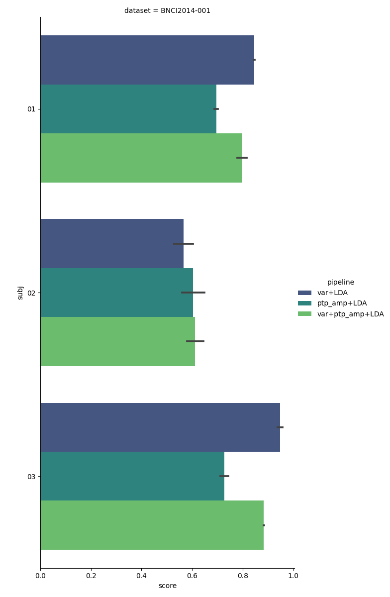
The following plot shows a comparison of the three classification pipelines for each subject. We can see that subjects 1 and 3, the pipeline using only the variance performs best. Perhaps this is because the variance is less sensitive to noise than the peak-to-peak amplitude, as the variance is computed over the whole epoch, whereas the peak-to-peak amplitude only considers the two most extreme data points (which could be outliers). For subject 2, the peak-to-peak amplitude pipeline works best.

In general, the pipeline using both peak-to-peak amplitude and variance has a mediocre performance, never beating the best single-feature pipeline in this experiment. This might be because using both variance and peak-to-peak amplitude increases the data dimensionality, without adding a lot of new information, resulting in increased overfitting.

results["subj"] = [str(resi).zfill(2) for resi in results["subject"]]
g = sns.catplot(
    kind="bar",
    x="score",
    y="subj",
    hue="pipeline",
    col="dataset",
    height=12,
    aspect=0.5,
    data=results,
    orient="h",
    palette="viridis",
)
plt.show()

References

[1] (1,2)

Schiratti, J. B., Le Douget, J. E., Le Van Quyen, M., Essid, S., & Gramfort, A. (2018, April). An ensemble learning approach to detect epileptic seizures from long intracranial EEG recordings. In 2018 IEEE International Conference on Acoustics, Speech and Signal Processing (ICASSP) (pp. 856-860). IEEE.

Estimated memory usage: 763 MB