

Note
Go to the end to download the full example code.
Tutorial: Within-Session Splitting on Real MI Dataset#
# Authors: Thomas, Kooiman, Radovan Vodila, Jorge Sanmartin Martinez, and Paul Verhoeven
#
# License: BSD (3-clause)
The justification and goal for within-session splitting#
In short, because we want to prevent the model from recognizing the subject and learning subject-specific representations instead of focusing on the task at hand.
In brain-computer interface (BCI) research, careful data splitting is critical. A naive train_test_split can easily lead to misleading results, especially in small EEG datasets, where models may accidentally learn to recognize subjects instead of decoding the actual brain task. Each brain produces unique signals, and unless we’re careful, the model can exploit these as shortcuts — leading to artificially high test accuracy that doesn’t generalize in practice.
To avoid this, we use within-session splitting, where training and testing are done on different trials from the same session. This ensures the model is evaluated under commonly used, consistent conditions while still preventing overfitting to trial-specific noise.
This approach forms a critical foundation in the MOABB evaluation framework, which supports three levels of model generalization:
Within-session: test generalization across trials within a single session
Cross-session: test generalization across different recording sessions
Cross-subject: test generalization across different brains
Where Within-session and cross-session are generalized across the same subject, cross-subject is generalized between (groups of) subjects.
Each level decreases in specialization, moving from highly subject-specific models, to those that can generalize across individuals.
This tutorial focuses on within-session evaluation to establish a reliable baseline for model performance before attempting more challenging generalization tasks.
Importing the necessary libraries#
import warnings

import matplotlib.pyplot as plt

# Standard imports
import pandas as pd
import seaborn as sns

# MNE + sklearn for pipeline
from mne.decoding import CSP
from sklearn.discriminant_analysis import LinearDiscriminantAnalysis as LDA
from sklearn.pipeline import make_pipeline

import moabb

# MOABB components
from moabb.datasets import BNCI2014_001
from moabb.evaluations.splitters import WithinSessionSplitter
from moabb.paradigms import LeftRightImagery


# Suppress warnings and enable informative logging
warnings.filterwarnings("ignore")
moabb.set_log_level("info")
Load the dataset#
In this example we use 3 subjects of the moabb.datasets.BNCI2014_001 dataset.
dataset = BNCI2014_001()
dataset.subject_list = [1, 2, 3]
Extract data: epochs (X), labels (y), and trial metadata (meta)#
For this dataset we use the moabb.paradigms.LeftRightImagery paradigm.
Additionally, we use the get_data method to download, preprocess, epoch, and label the data.
paradigm = LeftRightImagery()
# This call downloads (if needed), preprocesses, epochs, and labels the data
X, y, meta = paradigm.get_data(dataset=dataset, subjects=dataset.subject_list)

# Inspect the shapes: X is trials × channels × timepoints; y is labels; meta is info
print("X shape (trials, channels, timepoints):", X.shape)
print("y shape (trials,):", y.shape)
print("meta shape (trials, info columns):", meta.shape)
print(meta.head())  # shows subject/session for each trial
X shape (trials, channels, timepoints): (864, 22, 1001)
y shape (trials,): (864,)
meta shape (trials, info columns): (864, 3)
   subject session run
0        1  0train   0
1        1  0train   0
2        1  0train   0
3        1  0train   0
4        1  0train   0
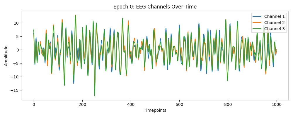
Visualising a single epoch.#
Plot a single epoch (e.g., the first trial), to see what’s in this dataset. (limiting to 3 channels for simplicity sake).
plt.figure(figsize=(10, 4))
plt.plot(X[0][0:3].T)  # Transpose to plot channels over time
plt.title("Epoch 0: EEG Channels Over Time")
plt.xlabel("Timepoints")
plt.ylabel("Amplitude")
plt.legend([f"Channel {i + 1}" for i in range(3)], loc="upper right")
plt.tight_layout()
plt.show()
Build a classification pipeline: CSP to LDA#
We use Common Spatial Patterns (CSP) finds spatial filters that maximize variance difference between classes. And then use Linear Discriminant Analysis (LDA) as a simple linear classifier on the extracted CSP features.
pipe = make_pipeline(
    CSP(n_components=6, reg=None),  # reduce to 6 CSP components
    LDA(),  # classify based on these features
)
pipe
Instantiate WithinSessionSplitter#
We want 5-fold cross-validation (CV) within each subject × session grouping
wss = WithinSessionSplitter(n_folds=5, shuffle=True, random_state=404)
print(f"Splitter config: folds={wss.n_folds}, shuffle={wss.shuffle}")

# How many total splits? equals n_folds × (num_subjects × sessions per subject)
total_folds = wss.get_n_splits(meta)
print("Total folds (num_subjects × sessions × n_folds):", total_folds)
# If wss is applied to a dataset where a subject has only one session,
# the splitter will skip that subject silently. Therefore, we raise an error.
if wss.get_n_splits(meta) == 0:
    raise RuntimeError("No splits generated: check that each subject has ≥2 sessions.")
Splitter config: folds=5, shuffle=True
Total folds (num_subjects × sessions × n_folds): 30
Manual evaluation loop: train/test each fold#
We’ll collect one row per fold: which subject/session was held out and its score
records = []
for fold_id, (train_idx, test_idx) in enumerate(wss.split(y, meta)):
    # Slice our epoch array and labels
    X_train, X_test = X[train_idx], X[test_idx]
    y_train, y_test = y[train_idx], y[test_idx]

    # Fit the CSP+LDA pipeline on the training fold
    pipe.fit(X_train, y_train)
    # Evaluate on the held-out trials
    score = pipe.score(X_test, y_test)

    # Identify which subject & session these test trials come from
    # (all test_idx in one fold share the same subject/session)
    subject_held = meta.iloc[test_idx]["subject"].iat[0]
    session_held = meta.iloc[test_idx]["session"].iat[0]

    # Record information for later analysis
    records.append(
        {
            "fold": fold_id,
            "subject": subject_held,
            "session": session_held,
            "score": score,
        }
    )

# Create a DataFrame of fold results
df = pd.DataFrame(records)

# Add a new column to indicate whether the data is train or test
df["split"] = df["session"].apply(lambda x: "test" if "test" in x else "train")

# Show the first few rows: one entry per fold
print(df.head())
   fold  subject session     score split
0     0        2   1test  0.620690  test
1     1        2   1test  0.724138  test
2     2        2   1test  0.586207  test
3     3        2   1test  0.413793  test
4     4        2   1test  0.714286  test
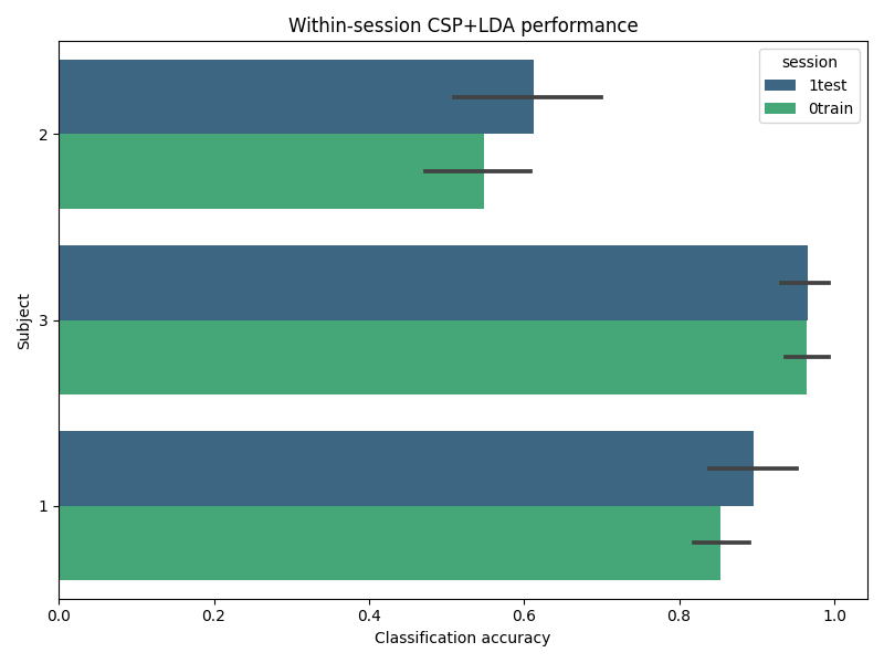
Summary of results#
We can quickly see per-subject, per-session performance: We see subject 2’s Session 1 has lower mean accuracy, suggesting session variability. Note: you could plot these numbers to visually compare sessions, but here we print them to focus on the splitting logic itself.
summary = df.groupby(["subject", "session"])["score"].agg(["mean", "std"]).reset_index()
print("\nSummary of within-session fold scores (mean ± std):")
print(summary)
Summary of within-session fold scores (mean ± std):
   subject session      mean       std
0        1  0train  0.853941  0.045977
1        1   1test  0.895567  0.073760
2        2  0train  0.549015  0.092128
3        2   1test  0.611823  0.125563
4        3  0train  0.965025  0.035110
5        3   1test  0.965517  0.042233
Visualisation of the results#
df["subject"] = df["subject"].astype(str)
plt.figure(figsize=(8, 6))
sns.barplot(x="score", y="subject", hue="session", data=df, orient="h", palette="viridis")
plt.xlabel("Classification accuracy")
plt.ylabel("Subject")
plt.title("Within-session CSP+LDA performance")
plt.tight_layout()
plt.show()
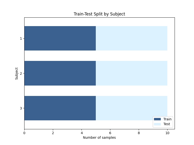
Visualisation of the data split#
For our 3 subjects, we see that each subject has 5 folds of training data.
def plot_subject_split(ax, df):
    """Create a bar plot showing the split of subject data into train and test."""
    colors = ["#3A6190", "#DDF2FF"]  # Colors for train and test

    # Count the number of train and test samples for each subject
    subject_counts = df.groupby(["subject", "split"]).size().unstack(fill_value=0)

    # Plot the train and test counts for each subject
    subject_counts.plot(
        kind="barh",
        stacked=True,
        color=colors,
        ax=ax,
        width=0.7,
    )

    ax.set(
        xlabel="Number of samples",
        ylabel="Subject",
        title="Train-Test Split by Subject",
    )
    ax.legend(["Train", "Test"], loc="lower right")
    ax.invert_yaxis()
    return ax


# Create a new figure for the subject split plot
fig, ax = plt.subplots(figsize=(8, 6))
# Add the subject split plot to the figure
plot_subject_split(ax, df)
<Axes: title={'center': 'Train-Test Split by Subject'}, xlabel='Number of samples', ylabel='Subject'>
Total running time of the script: (0 minutes 20.999 seconds)
Estimated memory usage: 743 MB